AIOmarRehan/resnet50v2-covid-xray-heatmap

ResNet50V2 COVID 19 Radiography Classification

Project Overview

This project builds a deep learning pipeline for chest X ray image classification using ResNet50V2 and transfer learning. The workflow covers data loading, exploratory data analysis, data cleaning, class balancing, preprocessing, model training, fine tuning, evaluation, Grad CAM explainability, and model export.

The repository includes a Gradio web application for interactive model predictions and Grad CAM visualizations, fully containerized with Docker for easy deployment.

Objectives

1. 1.Train a high quality medical image classifier using transfer learning.
2. 2.Improve class balance using augmentation driven oversampling.
3. 3.Evaluate performance with class level and aggregate metrics.
4. 4.Explain model decisions with Grad CAM visual analysis.
5. 5.Deploy predictions through an optimized and containerized Gradio application.

Repository Structure

1. 1.Notebook and Py File/ResNet50V2_COVID_19_Radiography.ipynb contains the end to end notebook workflow.
2. 2.Notebook and Py File/resnet50v2_covid_19_radiography.py contains the notebook exported as a Python script.
3. 3.saved_model/ResNet50V2_COVID-19_Radiography.h5 contains the trained model artifact.
4. 4.app/main.py contains Gradio interface for prediction and Grad CAM visualization.
5. 5.app/model.py contains model loading, prediction, and optimized Grad CAM utilities.
6. 6.Dockerfile specifies the containerized environment for deployment.
7. 7.docker-compose.yml orchestrates the containerized application.
8. 8.requirements.txt contains Python dependencies.

Methodology

1. Data Ingestion

The dataset is loaded from a compressed archive and converted into a tabular index with class label, file name, and full file path.

2. Exploratory Data Analysis

EDA is used to validate class distribution, image shape profile, channel profile, and data quality signals such as brightness and contrast.

3. Data Balancing and Augmentation

Class balancing is performed with ImageDataGenerator using geometric and photometric transforms. Minority classes are augmented to a target count to reduce class bias during training.

4. Data Cleaning

The pipeline checks for missing values, duplicates, corrupted files, file naming issues, outlier resolutions, and poor exposure cases.

<table align="center"> <tr> <td align="center"> <img src="https://files.catbox.moe/4p9v57.png" width="300" height="220"><br> <em><b>Percentage of Images per Class</b></em> </td> <td align="center"> <img src="https://files.catbox.moe/lhjnt9.png" width="300" height="220"><br> <em><b>Number of Images per Class</b></em> </td> </tr> <tr> <td align="center"> <img src="https://files.catbox.moe/wmovq0.png" width="300" height="220"><br> <em><b>Image Mode Distribution</b></em> </td> <td align="center"> <img src="https://files.catbox.moe/e6zfxv.png" width="300" height="220"><br> <em><b>Image Height Distribution</b></em> </td> </tr> <tr> <td align="center"> <img src="https://files.catbox.moe/nfbqun.png" width="300" height="220"><br> <em><b>Image Width Distribution</b></em> </td> <td align="center"> <img src="https://files.catbox.moe/ozfp7n.png" width="300" height="220"><br> <em><b>Class Distribution Check</b></em> </td> </tr> </table>

5. Preprocessing and Dataset Split

The preprocessing function decodes images, resizes to model input shape, normalizes pixel values, and applies controlled augmentation to the training stream. Data is split with stratification into training, validation, and test subsets.

6. Model Development

ResNet50V2 is used as a frozen feature extractor in phase one, followed by partial layer unfreezing for fine tuning in phase two. The classification head uses global average pooling, dense projection, dropout, and softmax output.

7. Evaluation

Performance is assessed using accuracy curves, loss curves, confusion matrix, classification report, precision, recall, F1 score, and ROC analysis.

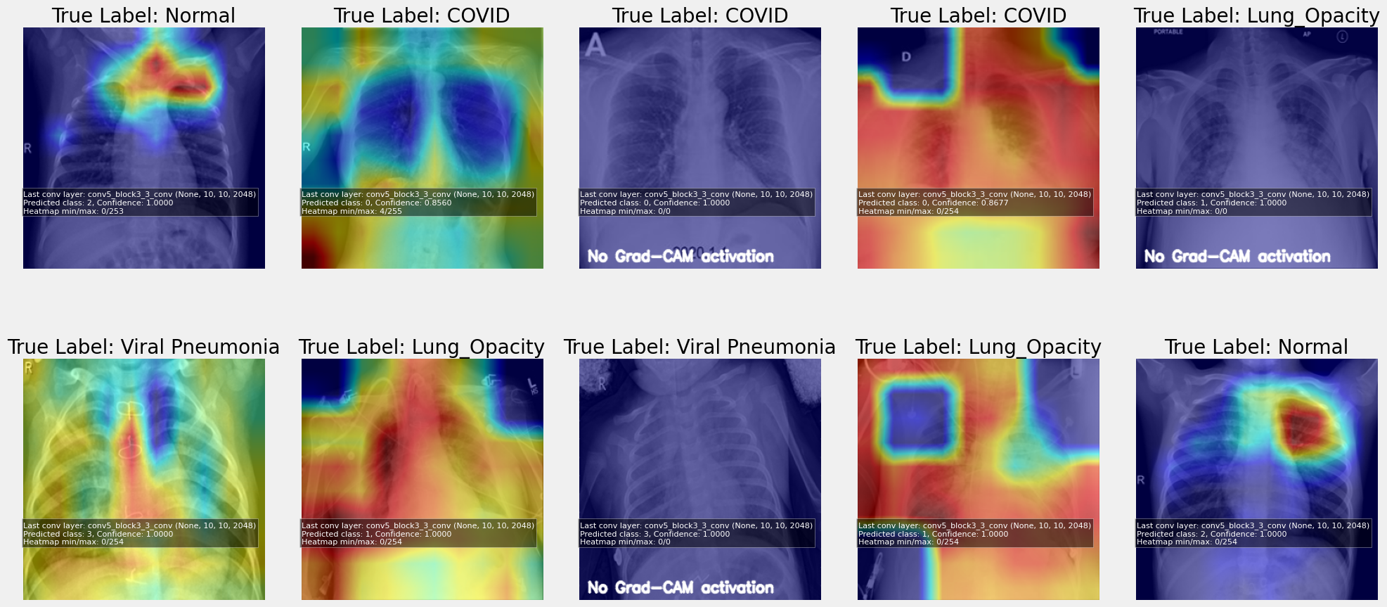
8. Explainability with Grad CAM

Grad CAM is generated from the final convolutional representation to highlight image regions that contribute to the predicted class.

9. Performance Optimization

Grad CAM computation was optimized through three key techniques: caching the Conv2D layer reference at startup, building the auxiliary gradient model once instead of reconstructing it per request, and compiling the gradient computation with TF function to enable graph mode execution. These changes reduce Grad CAM latency from approximately 16 seconds to 1-2 seconds per request after the first call.

Key Code Snippets

Data Index Construction

image_extensions = {'.jpg', '.jpeg', '.png'}
paths = [(path.parts[-2], path.name, str(path))
         for path in Path(extract_to).rglob('*.*')
         if path.suffix.lower() in image_extensions]

df = pd.DataFrame(paths, columns=['class', 'image', 'full_path'])

Preprocessing Function

def preprocess_image(path, target_size=(299, 299), augment=True):
    img = tf.io.read_file(path)
    img = tf.image.decode_image(img, channels=3)
    img.set_shape([None, None, 3])
    img = tf.image.resize(img, target_size)
    img = tf.cast(img, tf.float32) / 255.0

    if augment:
        img = tf.image.random_flip_left_right(img)
        img = tf.image.random_flip_up_down(img)
        img = tf.image.random_brightness(img, max_delta=0.1)
        img = tf.image.random_contrast(img, lower=0.9, upper=1.1)

    img = tf.clip_by_value(img, 0.0, 1.0)
    return img

Transfer Learning Model Head

resnet50v2 = ResNet50V2(input_shape=input_shape, weights='imagenet', include_top=False)

for layer in resnet50v2.layers:
    layer.trainable = False

x = GlobalAveragePooling2D()(resnet50v2.output)
x = Dense(512, activation='relu')(x)
x = Dropout(0.5)(x)
prediction = Dense(len(le.classes_), activation='softmax')(x)

model = Model(inputs=resnet50v2.input, outputs=prediction)

Training Callbacks

callbacks = [
    EarlyStopping(monitor='val_loss', patience=10, restore_best_weights=True, verbose=1),
    ModelCheckpoint('best_model.h5', save_best_only=True, monitor='val_loss', verbose=1),
    ReduceLROnPlateau(monitor='val_loss', factor=0.5, patience=5, min_lr=1e-5, verbose=1)
]

Grad CAM Invocation

overlay_img, info = VizGradCAM(model, img, interpolant=0.5, plot_results=False)

Setup and Installation

Docker Deployment (Recommended)

1. 1.Ensure Docker Desktop is running with the Linux engine enabled.
2. 2.Open a terminal in the project root.
3. 3.Run docker compose build to build the image.
4. 4.Run docker compose up -d to start the container.
5. 5.Open your browser to http://127.0.0.1:7860 to access the Gradio interface.

Useful Docker commands:

• —Stop container: docker compose down
• —View logs: docker compose logs -f
• —Rebuild after code changes: docker compose up --build -d

Local Environment (Alternative)

1. 1.Open a terminal in the project root.
2. 2.Run py -m venv venv.
3. 3.Run Set-ExecutionPolicy -ExecutionPolicy RemoteSigned -Scope Process.
4. 4.Run ./venv/Scripts/Activate.ps1.
5. 5.Run pip install -r requirements.txt.
6. 6.Run python -m app.main.
7. 7.Open your browser to http://127.0.0.1:7860 to access the Gradio interface.

Application Features

The Gradio interface provides:

1. 1.Image upload and preprocessing
2. 2.Real time class prediction with confidence scores
3. 3.Per class probability distribution
4. 4.Grad CAM visualization with adjustable interpolation (0.0 to 1.0)
5. 5.One click Run All button for complete analysis

Performance Notes

Prediction latency: Approximately 2 seconds per image on CPU.

Grad CAM latency: Approximately 1-2 seconds after the first call (5-6 seconds for the first call after container restart due to TF function JIT compilation).

Performance is optimized through caching of the gradient computation subgraph and use of TensorFlow function decoration for graph mode execution.

Consistency Checklist

1. 1.Keep dataset split random seed fixed.
2. 2.Keep class label encoder mapping fixed.
3. 3.Keep target image size fixed across training and inference (299x299).
4. 4.Keep normalization logic fixed across notebook and application code.
5. 5.Version model artifact with training configuration metadata.
6. 6.Verify that app/model.py points to the correct COVID radiography model artifact.
7. 7.Confirm that CLASS_NAMES order matches the label encoder order from training.

Results (Downloadable file)